
Old code refurbishment!
Introduction
Here are the general requirements for writing code:
- Code Readability:
- Use meaningful variable and function names so that others can understand what the code does.
- Utilize comments appropriately to explain complex algorithms or logic.
- Follow style guidelines such as indentation and spacing to keep the code neat and consistent.
- Modular Design:
- Break code down into small, reusable functions or modules, with each module responsible for a specific task.
- Avoid duplicate code by using functions or classes to reuse logic.
- Error Handling:
- Implement error handling mechanisms to ensure that the code can gracefully handle exceptions rather than crashing.
- Use exception handling to catch and manage potential errors.
- Performance Optimization:
- For applications with high performance requirements, pay attention to the time complexity and space complexity of algorithms.
- Collect and analyze performance data, and optimize as necessary.
- Testing:
- Write unit tests to ensure the correctness of each functional module.
- Use testing frameworks to automate the testing process and ensure that functionality is not broken after code changes.
- Documentation:
- Write project documentation to explain how to use, set up, and understand the functionalities of the code.
- Provide API documentation to help developers understand how to utilize your codebase.
- Version Control:
- Use version control tools (such as Git) to manage the history of code changes.
- Make clear commits with meaningful messages.
- Adhering to Best Practices:
- Always keep an eye on the best practices for the language and framework you are using, updating code to conform to the latest standards.
- Engage in code reviews to learn from colleagues and improve code quality.
Example One: Venn Diagram
Detailed content Click
- modified code
#!/usr/bin/env Rscript
# -*- coding: utf-8 -*-
# @Author    : mengqingyao
# @Time      : 20241029
# @File      : veen.r

library(readr)
library(tidyverse)
library(ggVennDiagram)
library(R6)

# 创建一个R6类
VennDiagramAnalysis <- R6Class("VennDiagramAnalysis",
  public = list(
    orthogroups_file = NULL,
    unassigned_genes_file = NULL,
    output_prefix = "venn_diagram",  # 输出前缀
    plot_width = 20,                  # 图片宽度
    plot_height = 18,                 # 图片高度
    Orthogroup_all = NULL,
    orth_gen = NULL,
    result = NULL,

    initialize = function(orthogroups_file, unassigned_genes_file, output_prefix = "venn_diagram", plot_width = 20, plot_height = 18) {
      self$orthogroups_file <- orthogroups_file
      self$unassigned_genes_file <- unassigned_genes_file
      self$output_prefix <- output_prefix
      self$plot_width <- plot_width
      self$plot_height <- plot_height
      self$load_data()
      self$process_data()
    },

    load_data = function() {
      Orthogroups <- read_tsv(self$orthogroups_file)
      Orthogroups_UnassignedGenes <- read_tsv(self$unassigned_genes_file)
      self$Orthogroup_all <- bind_rows(Orthogroups, Orthogroups_UnassignedGenes) %>%
        select(-"Hartmannula_sinica_185.fna_remove")
    },

    first_obse = function(data, n = 1, sep = ",") {
      list <- as.list(data)
      for (v in 2:length(colnames(data))) {
        for (o in 1:length(rownames(data))) {
          list[[v]][o] <- list[[v]][[o]] %>% strsplit(sep)
          list[[v]][o] <- list[[v]][[o]][n]
        }
      }
      for (v in 2:length(colnames(data))) {
        list[[v]] <- as.character(list[[v]])
      }
      as.data.frame(list)
    },

    process_data = function() {
      Orthogroup_all <- self$first_obse(self$Orthogroup_all)
      col_names <- colnames(Orthogroup_all)[-1]

      unique_symbols <- unique(gsub("[A-Za-z0-9]", "", col_names))
      split_content_list <- lapply(col_names, function(name) {
        strsplit(name, paste0("[", paste(unique_symbols, collapse = ""), "]"))[[1]]
      })

      col_renames <- sapply(split_content_list, function(split_content) {
        paste(head(split_content, 2), collapse = "_")
      })

      self$orth_gen <- lapply(seq_along(col_renames), function(i) {
        Orthogroup_all %>%
          filter(!!rlang::sym(col_names[i]) != "NA") %>%
          select(Orthogroup, !!rlang::sym(col_names[i])) %>%
          rename(!!col_renames[i] := "Orthogroup")
      })

      result <- Orthogroup_all %>% select(-Orthogroup)

      for (i in 1:length(col_names)) {
        result <- result %>%
          left_join(self$orth_gen[[i]], by = setNames(col_names[i], colnames(self$orth_gen[[i]])[2]))
      }

      self$result <- result %>% select((length(col_names) + 1):length(result))
    },

    plot_venn_diagram = function() {
      p1 <- ggVennDiagram(self$result, label = "count", edge_size = 1, label_alpha = 0) +
        scale_color_brewer(palette = "Set1") +
        scale_x_continuous(expand = expansion(mult = .2)) +
        scale_fill_distiller(palette = "Blues", direction = 1)

      p2 <- ggVennDiagram(self$result, label = "count", edge_size = 1, label_alpha = 0,
                          set_color = c("blue", "red", "green", "purple", "orange", "yellow", "cyan")) +
        scale_color_brewer(palette = "Set1") +
        scale_x_continuous(expand = expansion(mult = .2)) +
        scale_fill_distiller(palette = "Blues", direction = 1)

      # 使用输出前缀和尺寸进行保存
      ggsave(filename = paste0(self$output_prefix, "_p1.pdf"), plot = p1, width = self$plot_width, height = self$plot_height, units = "cm")
      ggsave(filename = paste0(self$output_prefix, "_p2.pdf"), plot = p2, width = self$plot_width, height = self$plot_height, units = "cm")
    }
  )
)
Save the above code to a file, e.g. veen.r
Now, let’s test the code:
source(veen.r)

venn_analysis <- VennDiagramAnalysis$new(
  orthogroups_file = "./OrthoFinder/OrthoFinder/Results_May31/Orthogroups/Orthogroups.tsv",
  unassigned_genes_file = "./OrthoFinder/OrthoFinder/Results_May31/Orthogroups/Orthogroups_UnassignedGenes.tsv",
  output_prefix = "my_venn_diagram",  # 自定义输出前缀
  plot_width = 25,                     # 自定义宽度
  plot_height = 20                      # 自定义高度
)

venn_analysis$plot_venn_diagram()
The output will be two pdf files: my_venn_diagram_p1.pdf and my_venn_diagram_p2.pdf.
Example Two: Upset
Detailed content Click
#!/usr/bin/env Rscript
# -*- coding: utf-8 -*-
# @Author    : mengqingyao
# @Time      : 20241030

rm(list = ls())
library(readr)
library(ComplexUpset)
library(tidyverse)

Orthogroups <- read_tsv("./OrthoFinder/OrthoFinder/Results_May31/Orthogroups/Orthogroups.tsv")
Orthogroups_UnassignedGenes <- read_tsv("./OrthoFinder/OrthoFinder/Results_May31/Orthogroups/Orthogroups_UnassignedGenes.tsv")

# 最多支持7个变量
Orthogroups <- Orthogroups %>% select(-`Hartmannula_sinica_185.fna_remove`)
Orthogroups_UnassignedGenes <- Orthogroups_UnassignedGenes %>% select(-`Hartmannula_sinica_185.fna_remove`)

first_obse = function(data, n = 1, sep = ",") {
  list <- as.list(data)
  for (v in 2:length(colnames(data))) {
    for (o in 1:length(rownames(data))) {
      list[[v]][o] <- list[[v]][[o]] %>% strsplit(sep)
      list[[v]][o] <- list[[v]][[o]][n]
    }
  }
  for (v in 2:length(colnames(data))) {
    list[[v]] <- as.character(list[[v]])
  }
  as.data.frame(list)
}

Orthogroups <- first_obse(Orthogroups)
Orthogroups_all <- rbind(Orthogroups,Orthogroups_UnassignedGenes)

#  eggnog注释信息

all_7_species_emapper_mod <- read_delim("eggNOG_test/7_species.emapper_mod.annotations",
                                        delim = "\t", escape_double = FALSE,
                                        trim_ws = TRUE)

#  KASS注释信息
# 设置文件夹路径
kegg_path <- "./KEGG_test"  # 请替换为您的KEGG文件夹的实际路径

# 列出KEGG文件夹中的所有文件
kegg_files <- list.files(kegg_path)

# 识别唯一的符号
unique_symbols <- unique(gsub("[A-Za-z0-9]", "", kegg_files))

# 按符号全部分割
split_content_list <- lapply(kegg_files, function(name) {
  strsplit(name, paste0("[", paste(unique_symbols, collapse = ""), "]"))[[1]]
})

# 保留分割后的前两部分,“_”连接、
kegg_files_mod_1 <- sapply(split_content_list, function(split_content) {
  paste(head(split_content, 2),collapse = "_")
})

kegg_files_mod_2 <- sapply(split_content_list, function(split_content) {
  # 取前两个元素
  first_two <- head(split_content, 2)
  # 用paste将它们组合,并添加"_KO"(确保不重复)
  result <- paste(first_two, collapse = "_")
  # 确保只添加一个"_KO"
  if (!grepl("_KO$", result)) {  # 检查是否以"_KO"结尾
    result <- paste(result, "_KO", sep = "")
  }
  return(result)
})

kegg_files_mod_3 <- sapply(split_content_list, function(split_content) {
  first_two <- head(split_content, 2)
  result <- paste(first_two, collapse = "_")
  if (!grepl("_COG$", result)) {  # 检查是否以"_KO"结尾
    result <- paste(result, "_COG", sep = "")
  }
  return(result)
})

kegg_files_mod_4 <- sapply(split_content_list, function(split_content) {
  first_two <- head(split_content, 2)
  result <- paste(first_two, collapse = "_")
  if (!grepl("_merge$", result)) {  # 检查是否以"_KO"结尾
    result <- paste(result, "_merge", sep = "")
  }
  return(result)
})

kegg_files_mod_5 <- sapply(split_content_list, function(split_content) {
  first_two <- head(split_content, 2)
  result <- paste(first_two, collapse = "_")
  if (!grepl("_pre$", result)) {  # 检查是否以"_KO"结尾
    result <- paste(result, "_pre", sep = "")
  }
  return(result)
})

# 读取文件
kegg_list <- list()  # 确保 kegg_list 已初始化

for (i in 1:length(kegg_files)) {
  # 读取文件
  kegg_list[[i]] <- read_delim(paste("KEGG_test/", kegg_files[i], sep = ""),
                               delim = "\t",
                               escape_double = FALSE,
                               col_names = FALSE,
                               trim_ws = TRUE)

  # 修改列名
  names(kegg_list[[i]])[1] <- "query"
  names(kegg_list[[i]])[2] <- kegg_files_mod_1[i]  # 使用正确的 kegg_files_mod

  # 添加新的列,符合 dplyr 的用法
  kegg_list[[i]] <- kegg_list[[i]] %>%
    mutate(!!sym(kegg_files_mod_2[i]) := 1)  # 使用 !!sym() 确保列名正确

}

ann_gene_asso <- data.frame()

ann_gene_asso <- Reduce(function(x, y) merge(x, y, by = "query", all = TRUE),
                        kegg_list)

ann_gene_asso <- merge(all_7_species_emapper_mod, ann_gene_asso, by = "query", all = TRUE)

ann_gene_asso <- ann_gene_asso %>% select(query,`eggNOG_OGs`,all_of(kegg_files_mod_1), all_of(kegg_files_mod_2))

#  分离单个物种
results_separate <- lapply(1:length(kegg_files_mod_2), function(i) {
  ann_gene_asso %>%
    filter(get(kegg_files_mod_2[i]) == 1) %>%
    select(query, eggNOG_OGs, !!sym(kegg_files_mod_1[i]))  %>% # 使用 !!sym() 动态获取列名
    mutate(!!kegg_files_mod_5[i] := 1)
})
Orthogroups_all_names <- sort(names(Orthogroups_all)[-1])

dataframe_list <- lapply(seq_along(Orthogroups_all_names), function(i) {
  # 检查当前的列名
  left_col_name <- Orthogroups_all_names[i]

  if (!left_col_name %in% colnames(Orthogroups_all)) {
    stop(paste("Column", left_col_name, "not found in Orthogroups_all"))
  }

  Orthogroups_all %>%
    left_join(results_separate[[i]], by = setNames("query", Orthogroups_all_names[i])) %>%
    select(-all_of(Orthogroups_all_names)) %>%
    rename(!!kegg_files_mod_3[i] := eggNOG_OGs)
})

#  使用bind_rows合并列表中的所有数据框
combined_df <- bind_rows(dataframe_list)
combined_df <- combined_df %>% arrange(Orthogroup)

# 使用 dplyr 进行分组和串联
results_df <- combined_df %>%
  group_by(Orthogroup) %>%
  summarize(across(everything(), ~ paste(na.omit(.), collapse = ", ")), .groups = 'drop')

results_df[results_df == ""] <- NA

results_df <- results_df %>%
  mutate(across(-1, ~ ifelse(is.na(.), 0, 1)))

results_class <- results_df %>%
  mutate(
    classification = case_when(
      rowSums(across(ends_with("_COG"), ~ as.numeric(as.character(.)))) >= 1 &
        rowSums(across(all_of(kegg_files_mod_1), ~ as.numeric(as.character(.)))) >= 1 ~ "COG and KEGG",  # 首先检查同时存在 COG 和 KEGG 的情况
      rowSums(across(ends_with("_COG"), ~ as.numeric(as.character(.)))) >= 1 ~ "COG",
      rowSums(across(-c(ends_with("_COG"), Orthogroup), ~ as.numeric(as.character(.)))) >= 1 ~ "KEGG",
      rowSums(across(-Orthogroup, ~ as.numeric(as.character(.)))) == 0 ~ "Unknown",
      TRUE ~ "Other"
    )
  )

results_class_1 <- results_class  # 复制原始数据框

# 逐个处理每对列并生成新列
for (i in seq_along(kegg_files_mod_1)) {
  results_class_1 <- results_class_1 %>%
    mutate(!!kegg_files_mod_4[i] := ifelse(
      rowSums(across(c(kegg_files_mod_3[i], kegg_files_mod_1[i])),
              na.rm = TRUE) >= 1,
      1,
      0
    ))
}

results_class_1 <- results_class_1 %>%
  select(-all_of(c(kegg_files_mod_3, kegg_files_mod_1, kegg_files_mod_4)))

#  增加颜色映射
CC <- c(`COG` = '#3C5488B2', `COG and KEGG` = '#4DBBD5B2', `KEGG` = '#FF3333', `Unknown` = '#DDDDDD')

#  画图
p1 <- upset(results_class_1,
            kegg_files_mod_5,
            width = .1,
            wrap = T,
            min_size = 29,
            #  按照交集类型和交集大小排列
            sort_intersections_by=c('degree', 'cardinality'),
            base_annotations = list(
              "intersection size" = intersection_size(
                counts = T,
                mapping = aes(fill=classification)
              )
              +theme(axis.line.y = element_line(colour = "black",size=0.5),axis.ticks.y=element_line(colour = "black",size=0.5))+
                scale_y_continuous(expand = c(0,0))+
                scale_fill_manual(values = CC)
            ),
            set_sizes=(
              upset_set_size()+ geom_text(aes(label=..count..), hjust=1, stat='count')
              + expand_limits(y=2300)
              + theme(axis.text.x=element_text(angle=90))
            ))

ggsave(filename = "test.pdf", p1, width = 35, height = 20, units = "cm")
result
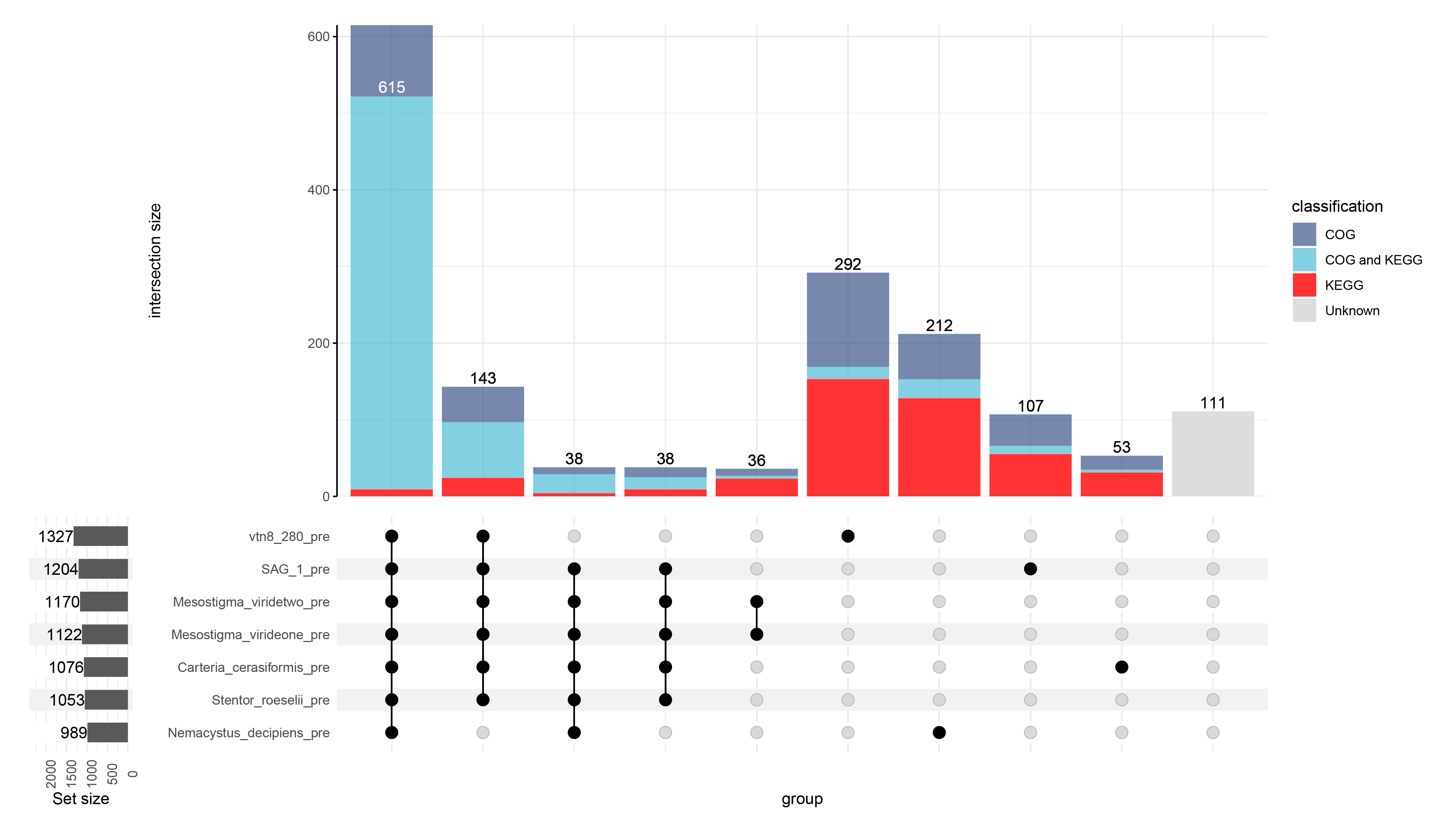
In the case of unknown genes that were not assigned to species, it is because for the homozygous gene analysis I used 8 species, and in this analysis I removed one.
Email me with more questions! 584338215@qq.com