Veen: OrthoFinder Results！

Introduction

A Venn diagram is a graphical representation used to visualize the overlapping regions of sets of elements. This diagram represents different sets through the use of closed curves (usually circles) and shows the intersection relationships between these sets through the overlapping parts between them. Venn diagrams have a wide range of applications in mathematics and logic, especially in set theory, for representing and analyzing various relationships between sets, such as intersection, concatenation, and complementary sets.

OrthoFinder used and result illustrated in this post. Click

Data from several bacteria OrthoFinder analysis results used to plot the veen diagram.

Data preparation

• All the data needed for the drawing of the veen diagram.

Now, let’s draw the Venn diagram

#!/usr/bin/env Rscript
# -*- coding: utf-8 -*-
# @Author    : mengqingyao
# @Time      : 20230531

rm(list = ls())
library(readr)
library(tidyfst)
library(tidyverse)
library(ggVennDiagram)

Orthogroups <-  read_tsv("./OrthoFinder/OrthoFinder/Results_May31/Orthogroups/Orthogroups.tsv") 

Orthogroups_UnassignedGenes <- read_tsv("./OrthoFinder/OrthoFinder/Results_May31/Orthogroups/Orthogroups_UnassignedGenes.tsv")

Orthogroup_all <- rbind(Orthogroups,Orthogroups_UnassignedGenes) %>% select_dt(-"Hartmannula_sinica_185.fna_remove")
#Orthogroup_all %>% count_dt(Orthogroup) 

Orthogroup_all <- separate_dt(Orthogroup_all, "Carteria_cerasiformis_72.fna_remove", c("Carteria_cerasiformis_1","Carteria_cerasiformis_2","Carteria_cerasiformis_3","Carteria_cerasiformis_4","Carteria_cerasiformis_5"), sep = ",")
Orthogroup_all <- separate_dt(Orthogroup_all, "Mesostigma_viride_28.fna_remove", c("Mesostigma_viride_28_1","Mesostigma_viride_28_2","Mesostigma_viride_28_3","Mesostigma_viride_28_4","Mesostigma_viride_28_5","Mesostigma_viride_28_6","Mesostigma_viride_28_7","Mesostigma_viride_28_8"), sep = ",")
Orthogroup_all <- separate_dt(Orthogroup_all, "Mesostigma_viride_1.fasta_remove", c("Mesostigma_viride_1_1","Mesostigma_viride_1_2","Mesostigma_viride_1_3","Mesostigma_viride_1_4","Mesostigma_viride_1_5","Mesostigma_viride_1_6","Mesostigma_viride_1_7","Mesostigma_viride_1_8","9","Mesostigma_viride_1_10"), sep = ",")
Orthogroup_all <- separate_dt(Orthogroup_all, "Nemacystus_decipiens_23.fna_remove", c("Nemacystus_decipiens_1","Nemacystus_decipiens_2","Nemacystus_decipiens_3","Nemacystus_decipiens_4","Nemacystus_decipiens_5","Nemacystus_decipiens_6","Nemacystus_decipiens_7","Nemacystus_decipiens_8","Nemacystus_decipiens_9","Nemacystus_decipiens_10","Nemacystus_decipiens_11","Nemacystus_decipiens_12","Nemacystus_decipiens_13"), sep = ",")
Orthogroup_all <- separate_dt(Orthogroup_all, "SAG_1.fna_remove", c("SAG_1","SAG_2","SAG_3","SAG_4","SAG_5","SAG_6" , "SAG_7",  "SAG_8"  ,"SAG_9" , "SAG_10", "SAG_11", "SAG_12" ,"SAG_13",
                                                                     "SAG_14" ,"SAG_15", "SAG_16", "SAG_17" ,"SAG_18" ,"SAG_19" ,"SAG_20" ,"SAG_21", "SAG_22" ,"SAG_23" ,"SAG_24", "SAG_25", "SAG_26",
                                                                     "SAG_27", "SAG_28", "SAG_29", "SAG_30" ,"SAG_31", "SAG_32", "SAG_33" ,"SAG_34" ,"SAG_35" ,"SAG_36", "SAG_37", "SAG_38" ,"SAG_39",
                                                                     "SAG_40" ,"SAG_41" ,"SAG_42","SAG_43","SAG_44","SAG_45","SAG_46","SAG_47","SAG_48","SAG_49","SAG_50","SAG_51","SAG_52","SAG_53"), sep = ",")
Orthogroup_all <- separate_dt(Orthogroup_all, "Stentor_roeselii_82.fna_remove", c("Stentor_roeselii_1","Stentor_roeselii_2","Stentor_roeselii_3","Stentor_roeselii_4","Stentor_roeselii_5","Stentor_roeselii_6","Stentor_roeselii_7","Stentor_roeselii_8"), sep = ",")
Orthogroup_all <- separate_dt(Orthogroup_all, "vtn8_280.fasta_remove", c("vtn8_1","vtn8_2","vtn8_3","vtn8_4","vtn8_5","vtn8_6","vtn8_7","vtn8_8","vtn8_9"), sep = ",")

Orthogroup_all <- Orthogroup_all %>% select_dt(Orthogroup,Carteria_cerasiformis_1,Mesostigma_viride_28_1,Mesostigma_viride_1_1,Nemacystus_decipiens_1,SAG_1,Stentor_roeselii_1,vtn8_1)
Orthogroup_all %>% count_dt(Orthogroup)


#  去除NA值，得到假基因和直系同源基因的对应关系
Carteria_cerasiformis_1 <- Orthogroup_all %>% filter_dt(Carteria_cerasiformis_1 != "NA") %>% 
  select_dt(Orthogroup,Carteria_cerasiformis_1) 
colnames(Carteria_cerasiformis_1)[1] <- "Carteria cerasiformis"

Mesostigma_viride_28_1 <- Orthogroup_all %>% filter_dt(Mesostigma_viride_28_1 != "NA") %>% 
  select_dt(Orthogroup,Mesostigma_viride_28_1) 
colnames(Mesostigma_viride_28_1)[1] <- "Mesostigma viride_28"

Mesostigma_viride_1_1 <- Orthogroup_all %>% filter_dt(Mesostigma_viride_1_1 != "NA") %>% 
  select_dt(Orthogroup,Mesostigma_viride_1_1) 
colnames(Mesostigma_viride_1_1)[1] <- "Mesostigma viride_1"

Nemacystus_decipiens_1 <- Orthogroup_all %>% filter_dt(Nemacystus_decipiens_1 != "NA") %>% 
  select_dt(Orthogroup,Nemacystus_decipiens_1) 
colnames(Nemacystus_decipiens_1)[1] <- "Nemacystus decipiens"

SAG_1 <- Orthogroup_all %>% filter_dt(SAG_1 != "NA") %>% 
  select_dt(Orthogroup,SAG_1) 
colnames(SAG_1)[1] <- "Cryptomonas gyropyrenoidosa"

Stentor_roeselii_1 <- Orthogroup_all %>% filter_dt(Stentor_roeselii_1 != "NA") %>% 
  select_dt(Orthogroup,Stentor_roeselii_1) 
colnames(Stentor_roeselii_1)[1] <- "Stentor roeselii"

vtn8_1 <- Orthogroup_all %>% filter_dt(vtn8_1 != "NA") %>% 
  select_dt(Orthogroup,vtn8_1) 
colnames(vtn8_1)[1] <- "E. octocarinatus VTN8"


result <- Orthogroup_all %>% select_dt(-Orthogroup)
result <- result %>% left_join(Carteria_cerasiformis_1,c("Carteria_cerasiformis_1" = "Carteria_cerasiformis_1"))
result <- result %>% left_join(Mesostigma_viride_28_1,c("Mesostigma_viride_28_1" = "Mesostigma_viride_28_1"))
result <- result %>% left_join(Mesostigma_viride_1_1,c("Mesostigma_viride_1_1" = "Mesostigma_viride_1_1"))
result <- result %>% left_join(Nemacystus_decipiens_1,c("Nemacystus_decipiens_1" = "Nemacystus_decipiens_1"))
result <- result %>% left_join(SAG_1,c("SAG_1" = "SAG_1"))
result <- result %>% left_join(Stentor_roeselii_1,c("Stentor_roeselii_1" = "Stentor_roeselii_1"))
result <- result %>% left_join(vtn8_1,c("vtn8_1" = "vtn8_1"))
result <- result %>% select_dt(`Carteria cerasiformis`, `Mesostigma viride_28`, `Mesostigma viride_1`, `Nemacystus decipiens`, `Cryptomonas gyropyrenoidosa`,`Stentor roeselii`, `E. octocarinatus VTN8`)

#  调色
#RColorBrewer::display.brewer.all()

#  作图
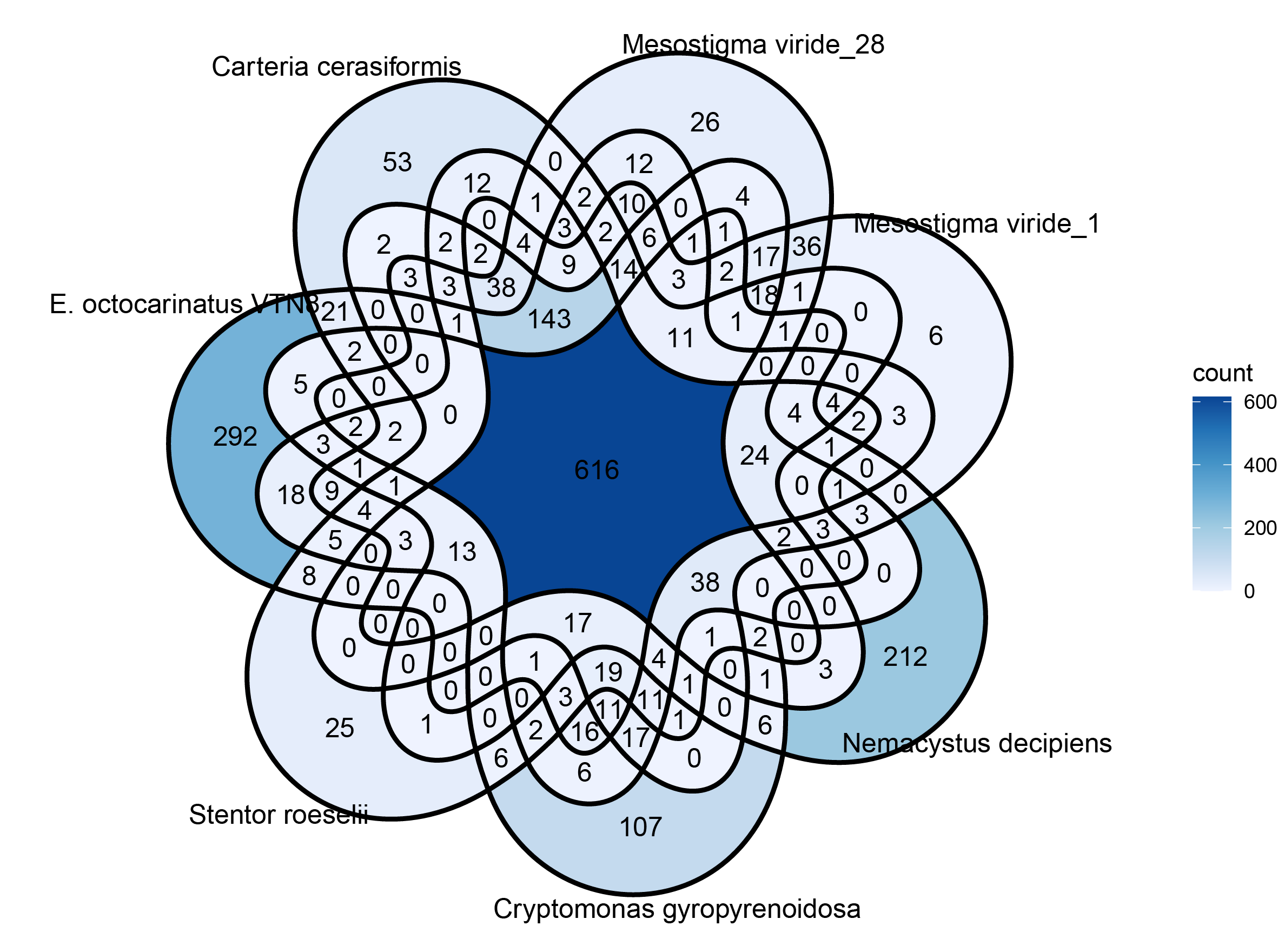
p1 <- ggVennDiagram(result, label = "count", edge_size = 1, label_alpha = 0) +
  scale_color_brewer(palette = "Set1") +
  scale_x_continuous(expand = expansion(mult = .2)) +
  scale_fill_distiller(palette = "Blues", direction = 1)

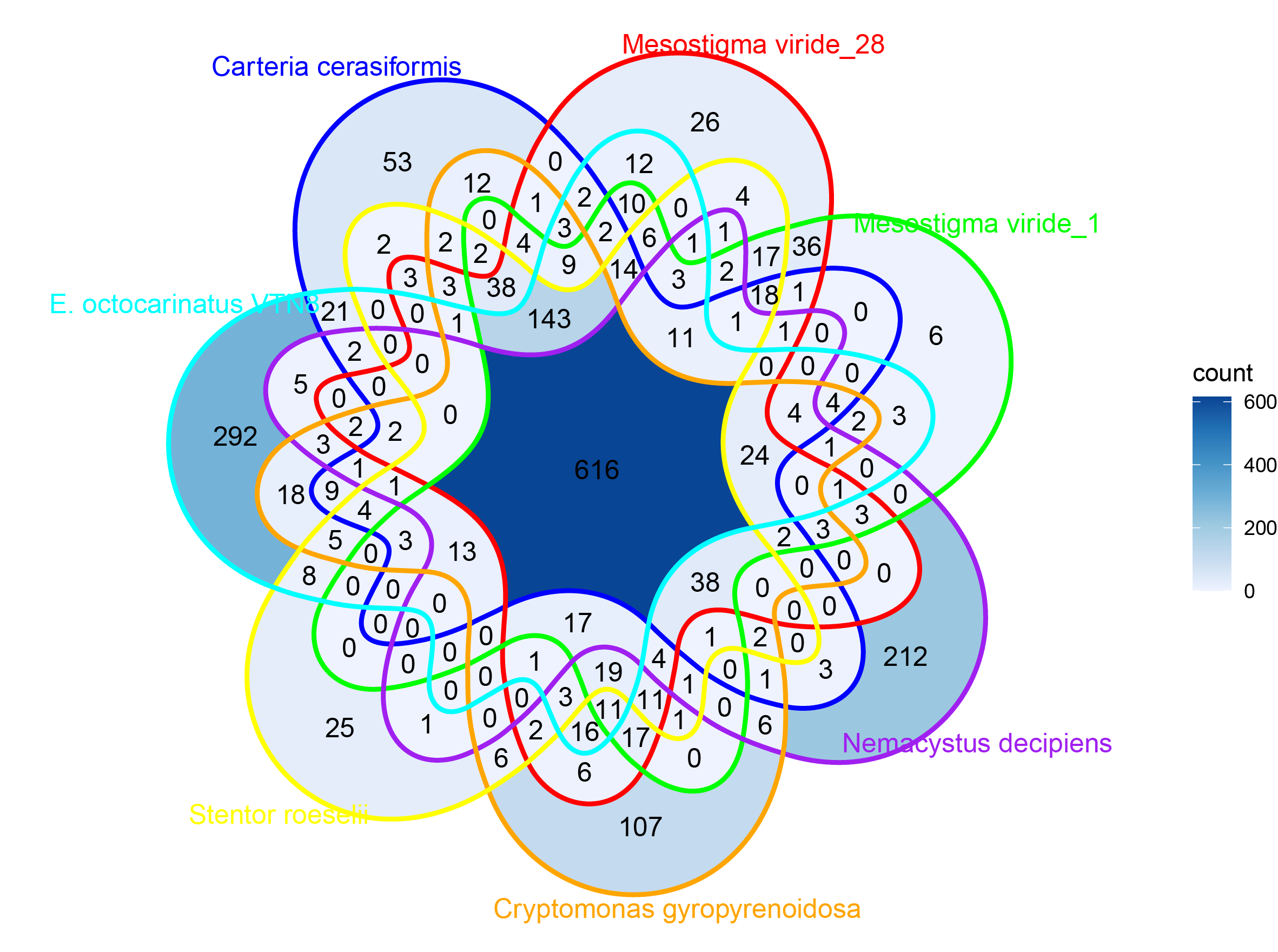
p2 <- ggVennDiagram(result, label = "count", edge_size = 1, label_alpha = 0, 
              set_color = c("blue", "red", "green", "purple", "orange", "yellow", "cyan")) +
  scale_color_brewer(palette = "Set1") +
  scale_x_continuous(expand = expansion(mult = .2)) +
  scale_fill_distiller(palette = "Blues", direction = 1)

ggsave(filename = "p1.pdf",p1, width = 20, height = 18, units = "cm")
ggsave(filename = "p2.pdf",p2, width = 20, height = 18, units = "cm")

Rsudio is recommended for running this script.

The above code has been updated. Click

I wrote this script a long time ago, and there is a lot of redundant code, but this is the original processing logic.

It's better to understand.

Result

Beautification

1. I would suggest saving the image as a pdf.
2. Evolutionary landscaping using Adobe Illustrator.
3. Save images as needed.

Quote

• OrthoFinder
• Rsudio
• tidyverse
• ggVennDiagram

Email me with more questions! 584338215@qq.com