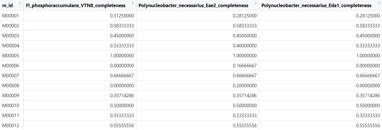
ggplot2: KEGG Modules Barplot!
Introduction
About KEGG module information and drawing data, please refer to the following link: Click
Data preparation


OK, let’s start!
#!/usr/bin/env Rscript
# -*- coding: utf-8 -*-
# @Author    : mengqingyao
# @Time      : 20231116


rm(list = ls())
library(readr)
library(tidyverse)
library(ggplot2)
library(tidyfst)

#  读取文件

#  绘制热图文件
# 游仆虫
eup_heatmap_file <- read_delim("tools_RStudio_result_all.txt",
                                       delim = "\t", escape_double = FALSE,
                                       trim_ws = TRUE)

# 必需共生菌
sym_heatmap_file <- read_delim("tools_RStudio_result_all_sym.txt",
                               delim = "\t", escape_double = FALSE,
                               trim_ws = TRUE)

#  去除多余变量
temp_1 <- sym_heatmap_file %>% select_dt(1:12)

#  生成筛选条件
filter_conditions <- paste0("temp_1$",names(temp_1)," != 0 & ",collapse ='')
filter_conditions <- substr(filter_conditions,0,nchar(filter_conditions)-3)
filter_conditions

#  去掉全部物种都为0的代谢模块
sym_heatmap_file <- sym_heatmap_file %>%
  filter_dt(temp_1$m_id != 0 & temp_1$Fl_phosphoraccumulans_VTN8_completeness != 0 & temp_1$Polynucleobacter_necessarius_Eae2_completeness != 0 & temp_1$Polynucleobacter_necessarius_Eda1_completeness != 0 & temp_1$Polynucleobacter_necessarius_Eae3_completeness != 0 & temp_1$Polynucleobacter_necessarius_Eae5_completeness != 0 & temp_1$Polynucleobacter_necessarius_Eco1_completeness != 0 & temp_1$Polynucleobacter_necessarius_Ewo1_completeness != 0 & temp_1$Polynucleobacter_necessarius_Eae1_completeness != 0 & temp_1$Polynucleobacter_necessarius_STIR1_completeness != 0 & temp_1$Polynucleobacter_necessarius_Fsp1.4_completeness != 0 & temp_1$Polynucleobacter_necessarius_amieti_completeness != 0) %>%
  select_dt(-1)

sym_heatmap_file$B_class[which(sym_heatmap_file$B_class == "Amino acid metabolism")] <- "Amino acid biosynthesis"
sym_heatmap_file$B_class[which(sym_heatmap_file$B_class == "Carbohydrate metabolism")] <- "Carbohydrates and lipid metabolism"
sym_heatmap_file$B_class[which(sym_heatmap_file$B_class == "Lipid metabolism")] <- "Carbohydrates and lipid metabolism"
sym_heatmap_file$B_class[which(sym_heatmap_file$B_class == "Glycan metabolism")] <- "Resistance and other"
sym_heatmap_file$B_class[which(sym_heatmap_file$B_class == "Biosynthesis of other secondary metabolites")] <- "Resistance and other"
sym_heatmap_file$B_class[which(sym_heatmap_file$B_class == "Glycan metabolism")] <- "Resistance and other"
sym_heatmap_file$B_class[which(sym_heatmap_file$B_class == "Nucleotide metabolism")] <- "Resistance and other"
sym_heatmap_file$B_class[which(sym_heatmap_file$B_class == "Biosynthesis of terpenoids and polyketides")] <- "Resistance and other"

#  游仆虫代谢模块数据处理 -------------------------------------------------------------
#  去除多余变量
eup_heatmap_file <- select(eup_heatmap_file, c(-m_id, -B_class))

#  寻找共有模块
Shared_metabolic_module <- sym_heatmap_file %>% left_join_dt(eup_heatmap_file)

#  去除多余变量
temp_1 <- Shared_metabolic_module %>% select_dt(-1,-13)

#  生成筛选条件
filter_conditions <- paste0("Shared_metabolic_module$",names(temp_1)," == 0 & ",collapse ='')
filter_conditions <- substr(filter_conditions,0,nchar(filter_conditions)-3)
filter_conditions

#  保存两种变量之间的排列信息
temp_1 <- Shared_metabolic_module %>% arrange_dt(B_class)

#write.table(Shared_metabolic_module,file = "Shared_metabolic_module.txt",sep = "\t", quote = F,row.names = F)

#  宽表变长表
Shared_metabolic_module <- Shared_metabolic_module %>% longer_dt('B_clas','m_name',name = "species",value = 'count')

#  将数据整理为绘图所需变量排序
Shared_metabolic_module <- Shared_metabolic_module %>% arrange_dt(B_class)

#  数据因子化,调整排列顺序
Shared_metabolic_module$B_class <- factor(Shared_metabolic_module$B_class, levels = c("Amino acid biosynthesis","Carbohydrates and lipid metabolism","Energy metabolism","Metabolism of cofactors and vitamins","Resistance and other"))
Shared_metabolic_module$m_name <- factor(Shared_metabolic_module$m_name, levels = rev(temp_1$m_name))

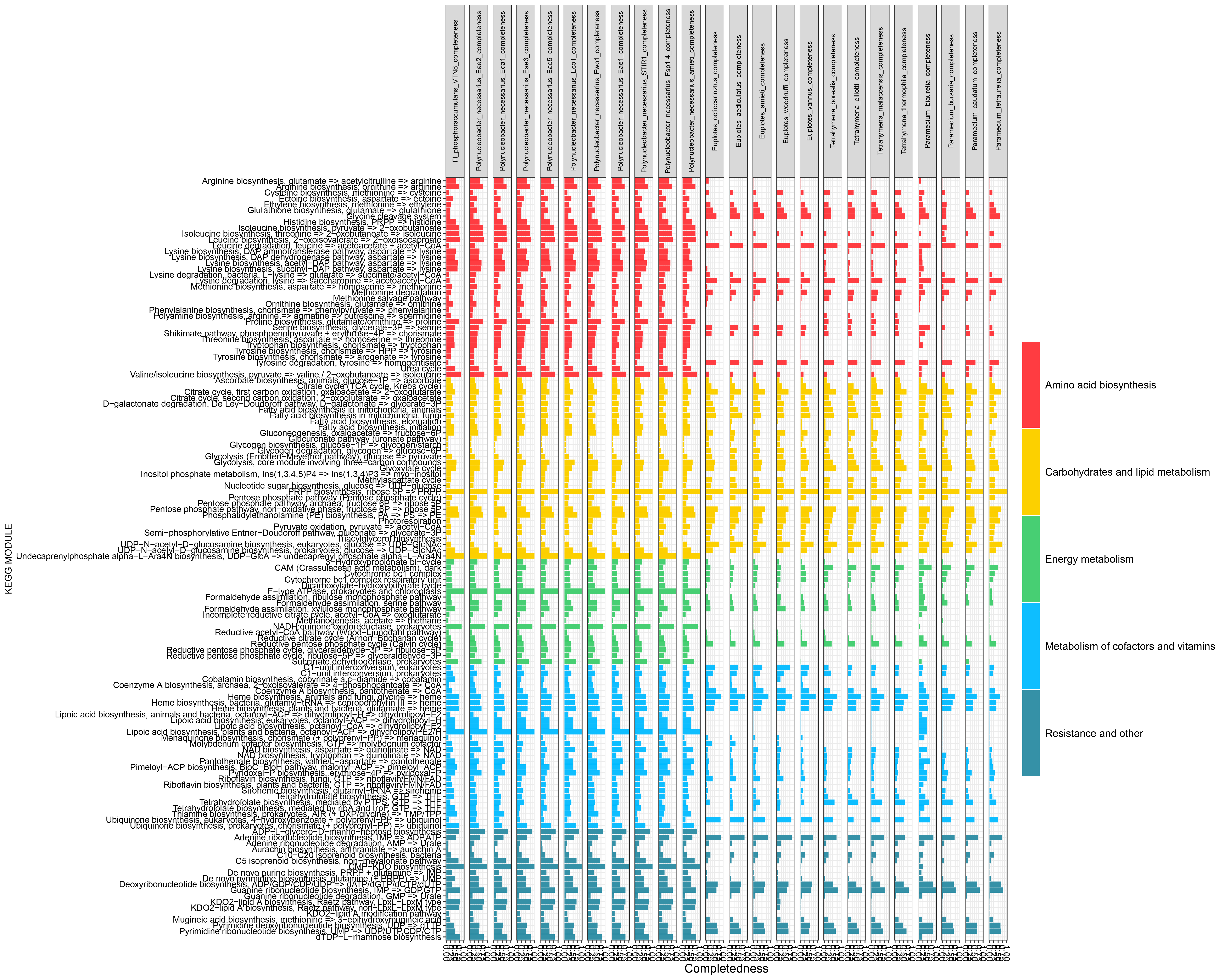
p1 <- ggplot(Shared_metabolic_module, aes(count, m_name, fill = B_class))+
  #绘制条形图函数
  geom_col()+
  #指定分面变量
  facet_grid(~species, scales = "free_x")+ #x轴随意变化
  #facet_wrap(~species)+
  #设置轴标题并去除图例的标题
  labs(fill=NULL, y = "KEGG MODULE", x = "Completedness")+
  #主题设置
  theme_bw()+
  theme(axis.text.y = element_text(size = 10, color = "black"),
        axis.text.x = element_text(size = 10, color = "black",
                                   angle = 270, vjust = 0.5, hjust = 0),
        strip.text = element_text(size = 8, color = "black",angle = 90),
        legend.text = element_text(size = 12, color = "black"),
        axis.title.x = element_text(size = 14, color = "black"))+
  #自定义颜色并设置图例长宽
  scale_fill_manual(values = c("#ff3c41","#fcd000","#47cf73","#0ebeff","#3591a7"),
                    guide=guide_legend(keywidth=1.5, keyheight=7))

ggsave(filename = "test.pdf", p1, width = 50, height = 40 ,units = "cm")
Rsudio is recommended for running this script.
I wrote this script a long time ago, and there is a lot of redundant code, but this is the original processing logic.
It's better to understand.
Result

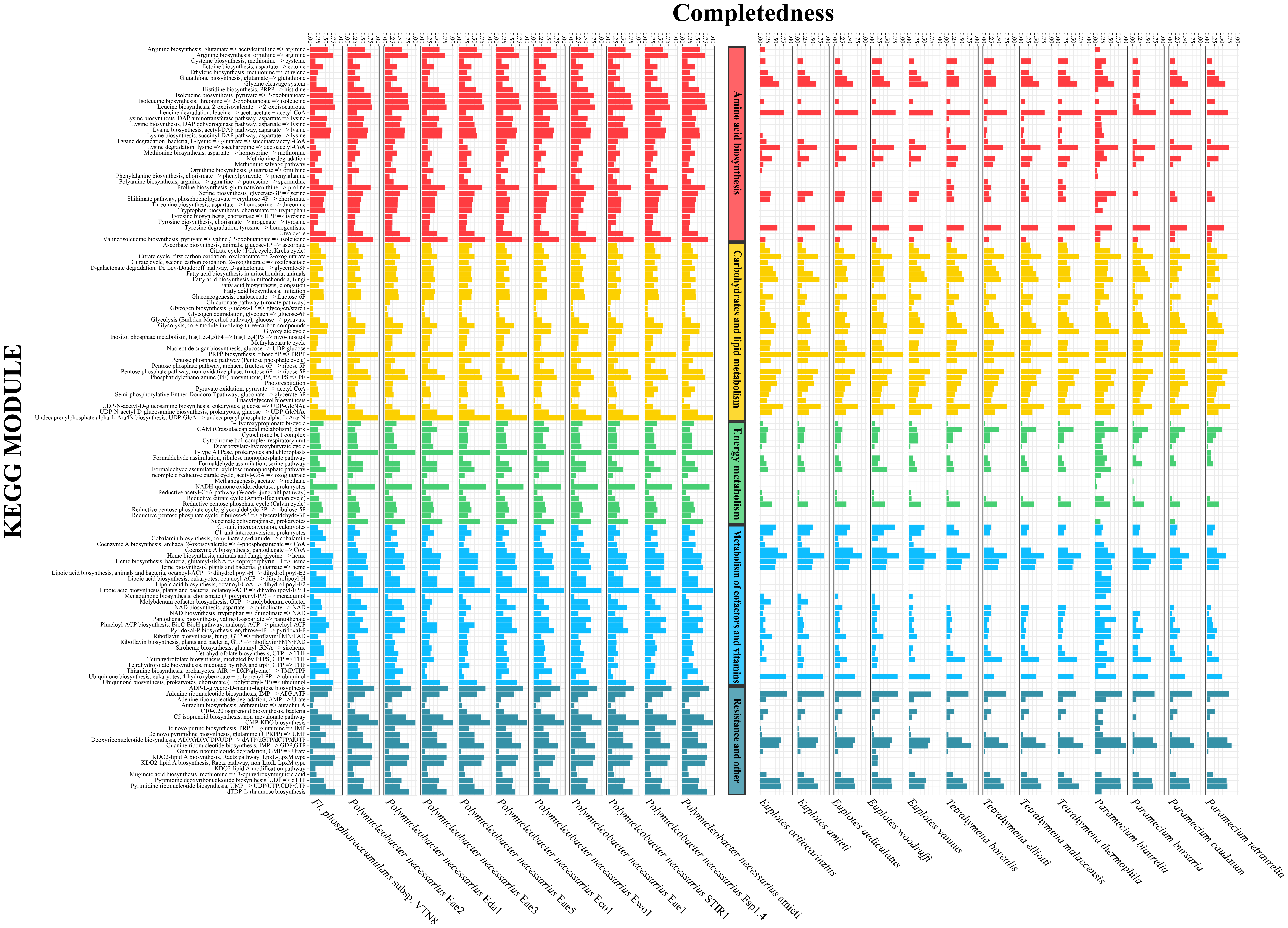
Beautification
- I would suggest saving the image as a pdf.
- Evolutionary landscaping using Adobe Illustrator.
- Save images as needed.

Quote
Email me with more questions! 584338215@qq.com
